
LPCTrap
The LPCTrap project is currently supported by the Conseil Régional de Normandie through the project THESMOG (Test of tHE Standard Model at Ganil, RIN Recherche N° 18E01660, 2018-2021).
Related project: MORA
The LPCTrap setup consists in a RFQ cooler-buncher and a transparent Paul Trap [1] (see figure 1). It is devoted to the measurement of the beta-neutrino angular correlation parameters a in the allowed transitions of nuclear ß decays. The aim of such experiments is twofold: either searching for “exotic” contributions to the weak interaction, beyond the V-A theory, in the case of pure (Fermi (F) or Gamow-Teller (GT)) transitions, or deducing, from the measurements of a, very precise values for the mixing ratios between the G-T and the F components, rho, in the case of mirror transitions. This enables to test the Conserved Vector Current (CVC) hypothesis and the unitarity of the Cabibbo-Kobayashi-Maskawa (CKM) matrix.
In these experiments, the ß particles are detected in coincidence with the recoiling ions and the coefficient a is deduced from the analysis of the time-of-flight (ToF) distribution of the latter relative to the ß’s. The recoil ions are detected with a spectrometer which is sensitive to their charge state distribution, also allowing the study of the shakeoff (SO) atomic process.
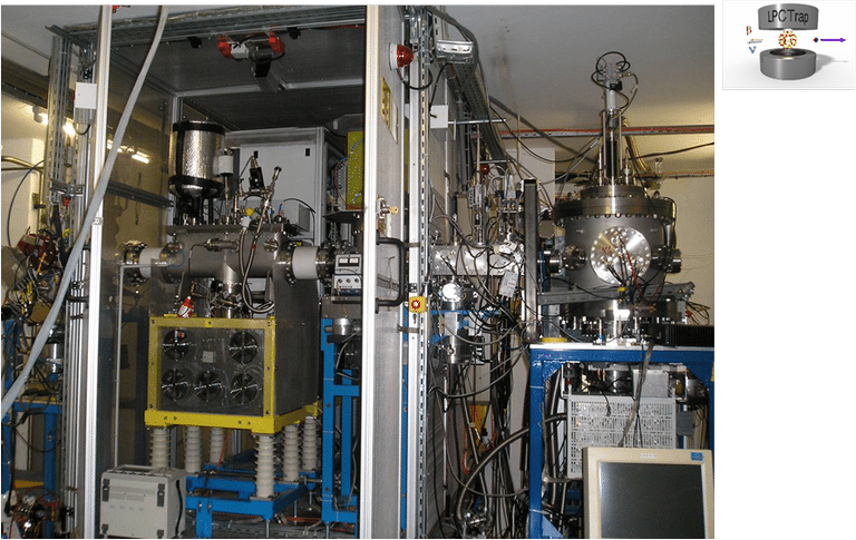
Figure 1 : The LPCTrap setup at LIRAT.
Experimental technique
The 1+ or 2+ ions, extracted from the SPIRAL target ion source system mounted at a potential of about 10 kV, are transported to the setup after a crude mass separation (delta M/M > 1/250). They are then cooled and bunched by means of the buffer gas technique with a Radio Frequency Quadrupole (RFQ) filled with H2 or He gas (left part of figure 2). More details about the operation of the RFQ can be found in [2].
Cold bunches of singly charged ions extracted from the RFQ are injected into the Paul trap (right part of figure 2). The transfer of ions from the RFQ, at high voltage, to the trap chamber at ground, is achieved with two pulsed cavities, located between the RFQ and the trap, which reduce the ion energy for an efficient trapping. The trap is made of a set of coaxial rings providing an open access for injection and extraction of ions and for the detection of the decay products. Ions are confined in the Paul trap by a RF field. The RF voltage is applied to the inner rings of the trap. The ß particles from in trap decays are detected by a telescope constituted by a double-sided position sensitive silicon strip detector (DSSD) followed by a thick plastic scintillator. The recoil ions are counted by a position sensitive micro-channel plate (µCP) [3]. In 2009, a recoil spectrometer was added in the setup to make it sensitive to the charge state distribution of the recoiling ions. This distribution enters in the systematic effects with an important weight when several electrons are involved. The setup is unique worldwide to measure such distributions in the case of singly charged ions decay. A second µCP, located downstream, serves to monitor the trapped ions and measures continuously the ions remaining in the trap at the end of the measurement cycle.
Ion bunches from the RFQ are continuously injected/extracted into/from the Paul trap, with a repetition rate of the order of 200 ms. The repetition rate is adjustable depending of the effective storage time of ions in the trap. After injection, the RF voltage is permanently applied to the rings of the Paul trap. The production of a signal by the plastic scintillator generates the trigger of an event, which in most cases is a ß particle in singles. Following a trigger, the DSSD is read out and a start signal is generated for the time measurement, waiting for a signal from the µCP over a time range of several µs adjusted to the energy range of the recoiling ions. For each coincidence event, the positions of both particles, the recoil ion ToF, the ß particle kinetic energy, the time stamp of the decay within the cycle and the RF phase of the trap are recorded. This set of measured parameters is useful to control systematic effects and to check the consistency of the results. In the cycle, the ions are kept during about 150 ms in the trap to study the decays, and they are ejected for the 50 ms left to study the background (Bg). This method enables to record a Bg sample at each cycle.

Figure 2: Details of the LPCTrap setup.
Achievements
Several runs were performed with 6He1+, 35Ar1+ and 19Ne2+ beams [4]. After a commissioning run in 2005, two experiments were performed in 2006 and 2010 with 6He+ ions. In the former, about 105 coincident events were recorded [5]. From a comparison of the time-of-flight spectrum to Monte Carlo simulations, the angular coefficient parameter could be determined with a statistical precision of 2 %. During the second experiment, about 1.2×10⁶ coincidences were recorded which would enable to reach a statistical precision of 0.6% on the measurement of a. To extract this coefficient from the data, realistic simulations are currently developed enabling to properly reproduce the response function of the whole setup and to study the systematic effects. Among them, the SO process has already been studied for this text book case, with only one electron (figure 3). Simple quantum calculations based on the sudden approximation could be tested with a relative precision better than 4×10⁻⁴ [6].
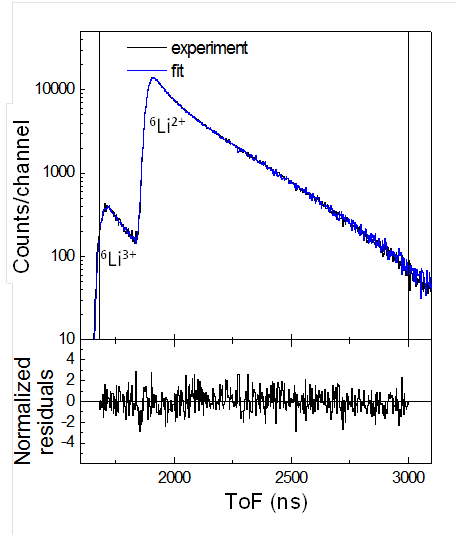
Figure 3: Fit of the experimental ToF spectrum to deduce the charge state distribution of the recoiling 6Li ions after the ß decay of trapped 6He+.
In 2011, a commissioning run performed with 35Ar+ ions has provided the charge state distribution of the recoiling 35Clq+ ions. The calculations, based on the Hartree-Fock method and on the sudden approximation, were found in excellent agreement with the experiment and showed a strong contribution of Auger electron emission [7]. During the second experiment performed in 2012, a total of 1.5×10⁶ coincidences were recorded (left part of figure 4). With such a statistics, the final result should constitute the most precise value ever obtained in a beta-neutrino angular correlation measurement.
In 2013, a first measurement was performed with 19Ne. In order to get rid of a huge contamination of the beam in stable mass 19, the LIRAT line was tuned for the 2+ charge state. By collision with the buffer gas at the entrance of LPCTrap, a large part of this beam quickly becomes singly charged allowing the tuning of the whole setup for 1+ ions. A total of 1.3×10⁵ coincidences were recorded (right part of figure 4). The charge state distribution of the 19Fq+ ions appears very different compared to that of 35Clq+ and is not satisfactorily reproduced by the current theoretical model, which seems to emphasize the limit of the independent particle model used in the theoretical approach [8]..
Some characteristics of these experiments are summarized in table 1.
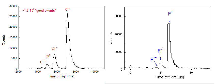
Figure 4: Experimental ToF spectra obtained during experiments performed with 35Ar+ (left panel) and 19Ne+ (right panel).
| Ion beam
(Half-life) |
Intensity (pps) |
Buffer gas |
LPCTrap OTE* (cycle) year |
Nb of coincidences | a (Delta atot)exp** | Ref. |
| 6He1+
(0.8 s) |
1.5×10⁸ | H2 | ~ 5×10⁻⁵
(100ms) 2006 ~ 5×10⁻⁴ (200ms) 2010 |
1.0×10⁵
1.2×10⁶ |
-0.334(10)
-0.3333(29)exp |
a: [5]
SO: [6] |
| 35Ar1+
(1.8 s) |
5.0×10⁷ | He | ~ 4×10⁻³
(200ms) 2012 |
1.5×10⁶ | 0.9004(26)exp | SO: [7] |
| 19Ne2+
(17.3 s) |
2.5×10⁸ | He | ~ 9×10⁻⁴
(200ms) 2013 |
1.3×10⁵ | 0.0364(89)exp | SO: [8] |
Table 1: Summary of main characteristics of experiments performed with 6He, 35Ar and 19Ne using LPCTrap at LIRAT. *: OTE = Overall Transmission Efficiency. **: exp = expected, when mentioned, the value in italic is an expected result.
References
[1] D. Rodriguez et al., Nucl. Instr. Meth. Phys. Res. A 565 (2006) 876.
[2] G. Ban et al., Nucl. Inst. Meth. Phys. Res. A 518 (2004) 712.
[3] E. Liénard et al., Nucl. Inst. Meth. Phys. Res. A 551 (2005) 375.
[4] E. Liénard et al., Hyp. Int. 236 (2015) 1.
[5] X. Fléchard et al., J. Phys. G: Nucl. Part. Phys. 38 (2011) 055101.
[6] C. Couratin et al., Phys. Rev. Lett. 108 (2012) 243201.
[7] C. Couratin et al., Phys. Rev. A 88 (2013) 041403(R).
[8] X. Fabian et al., Phys. Rev. A 97 (2018) 023402.
Other publications
X. Fléchard et al., Phys. Rev. Lett. 102 (2009) 125041.
X. Fléchard et al., Hyp. Int. 199 (2011) 21.
P. Velten et al., Hyp. Int. 199 (2011) 29.
G. Ban et al., Ann. Phys. 525 (2013) 576.
X. Fabian et al., EPJ Web Conferences 08002 (2014) 66.
X. Fabian et al., Hyp. Int. 235 (2015) 87.
Contact
Etienne Liénard, LPC Caen – lienard@lpccaen.in2p3.fr